How to Format ACCA Section C Spreadsheet Answers: 5 Mistakes That Cost You Distinction

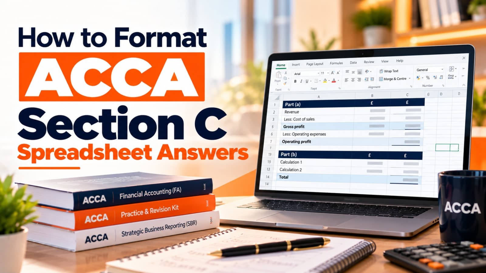
In ACCA Applied Skills and Strategic Professional examinations, Section C Constructive Response Questions (CRQs) account for 40% to 100% of total available marks. While most candidates spend hundreds of hours memorizing financial accounting standards, tax rules, and management theories, a surprising number fail or miss distinction scores (70%+) due to poor execution inside the official Computer Based Exam (CBE) spreadsheet workspace.

As an ACCA exam marker, I see hundreds of scripts where candidates know the underlying accounting principles, yet lose critical marks because their spreadsheets are chaotic, unformatted, hardcoded, or unreadable.

ACCA human markers do not just look at your final number; we grade your working logic, formula syntax, and layout structure.

Understanding how to construct clean, dynamic, and professional spreadsheet answers ensures you harvest every available method mark—even when your final calculated figure contains an early arithmetic error. Here is how to avoid the five most common spreadsheet formatting mistakes and format your Section C responses like a rank holder.

Understanding the ACCA CBE Spreadsheet Workspace

Before looking at specific formatting mistakes, you must understand the technical environment of the official ACCA CBE software. The ACCA spreadsheet tool is a custom, browser-based grid designed to mimic essential spreadsheet features, but it has distinct operational constraints compared to full commercial software like Microsoft Excel.

Key Constraints of the ACCA CBE Spreadsheet

• Single Worksheet Environment: Unlike Microsoft Excel, which allows multiple tabs/worksheets (Sheet1, Sheet2), the ACCA CBE spreadsheet gives you only one single worksheet per question. All workings, schedule tables, and narrative commentary must coexist on a single grid.

• Fixed Grid Structure: Adding or deleting rows and columns can shift unselected cells below or to the side, potentially disrupting adjacent tables. Master the use of cut-and-paste (Ctrl + X / Ctrl + V) to adjust layouts.

• Restricted Formula Library: While standard arithmetic operations (+, -, *, /) and core functions (=SUM, =AVERAGE, =NPV, =IRR, =SQRT, =ABS) work seamlessly, advanced Excel macros, custom scripts, and complex lookup functions are unsupported.

• Cell Inspection by Human Markers: When your script is submitted, human markers physically click into your response cells. We can see the exact formula string typed into the formula bar (e.g., =B5*C5).
  
  

Mistake 1: Hardcoding Calculated Values (Losing Method Marks)

The single most destructive habit in Section C is using a physical handheld calculator to compute numbers, then typing static, pre-calculated figures directly into spreadsheet cells.

When you type a static number like 131250 into a cell without a formula, the marker has no way of knowing how you arrived at that figure. If that number is incorrect—even by a single rupee or dollar due to a minor slip—you lose 100% of the marks for that line item and all downstream calculations.

The "Own Figure Rule" (OFR) Protection

ACCA markers apply the Own Figure Rule (OFR). Under OFR, if you make a mistake in Step 1 (e.g., miscalculating inflation rate), but you carry that wrong figure into Step 2 using a live cell reference formula (e.g., =B4 * C1), you receive full marks for Step 2. Hardcoding breaks this chain and destroys your OFR protection.

Hardcoding vs Dynamic Formulas

Marker's Gold Rule: Never type a number into a spreadsheet cell if that number can be calculated from other cells already present on your sheet!

Mistake 2: Misusing the Net Present Value (=NPV) Function Syntax

In Financial Management (FM) and Advanced Financial Management (AFM) papers, Investment Appraisal questions regularly require calculating Net Present Value (NPV). A widespread error involves misusing the syntax of the built-in =NPV() function inside the ACCA software.

The Standard Function Syntax Error

In standard financial modeling, the =NPV(rate, value1, [value2], ...) function assumes that value1 occurs at the end of Period 1 (Year 1).

Many candidates incorrectly include the Year 0 Initial Outlay inside the cash flow range argument:

INCORRECT:=NPV(0.10,C5:G5)(whereC5isYear0Outlay)

Because C5 is Year 0 (which occurs today at t0), including it inside the =NPV() range causes the software to discount your initial investment by 1 year at 10%, fundamentally corrupting your final NPV calculation.

The Correct NPV Formula Construction

Always separate Year 0 cash flows from the discounted range of Year 1 through Year N:

CORRECT:=NPV(Rate,Year1Range:YearNRange)+Year0Cell

Practical CBE Formula Syntax

Assuming Year 0 Outlay is in cell C5 (entered as a negative number) and Year 1 to Year 4 Net Cash Flows are in cells D5:G5, with the Cost of Capital (10%) in cell B2:

=NPV(B2, D5:G5) + C5

                         Correct NPV Formula Setup

                                      │

  Year 0 Cash Flow (t0) ──────────────┼──────────────► Add directly (Un-discounted)

  Cell C5 (-₹500,000)                 │                Formula: =NPV(B2, D5:G5) + C5

                                      │

  Years 1 to 4 Cash Flows ────────────┘

  Cells D5:G5 (Discounted at B2)

Mistake 3: Unformatted Data Walls & Missing Thousands Separators

ACCA markers grade hundreds of Section C submissions during marking windows. Presenting an unformatted grid filled with endless unaligned decimals and large numbers lacking commas creates an unreadable "data wall."

While markers try to trace candidate logic, poor formatting slows down evaluation, increases cognitive strain, and costs you presentation and layout marks.

4 Mandatory Formatting Rules

1. Apply Thousands Separators to Large Numbers

Always format monetary values using commas for thousands separators.

• Unformatted: 1250000 or 1250000.4567

• Formatted: 1,250,000

2. Standardize Decimal Precision Consistently

Never mix varying decimal lengths across the same calculation row.

• Currencies / Cash Flows: Round to the nearest whole integer or 2 decimal places (₹1,250.50).

• Discount Factors: Keep consistent at 3 decimal places (0.909, 0.826).

• Cost of Capital / Tax Rates: Keep consistent at 1 or 2 decimal places (10.0% or 10.5%).
  
  

3. Emphasize Key Sub-totals Using Bold (Ctrl + B)

Use keyboard shortcut Ctrl + B to highlight structural rows:

• Column Headers (e.g., Year 0, Year 1, Year 2)

• Key Row Sub-totals (e.g., Total Operating Costs, Taxable Profit)

• Final Line Items (e.g., Net Present Value (NPV), Revised Profit)

4. Establish Clear Column Headers and Unit Labels

Always state the currency unit and rounding scale explicitly in your table headers (e.g., All figures in ₹ '000 or All figures in $).

Mistake 4: Cramming Narrative Explanations Into Calculation Cells

Many Section C questions require a mix of numerical calculation and narrative justification (e.g., "Calculate the revised profit and discuss the impact on key performance indicators").

Candidates frequently make the mistake of typing text explanations directly into the same grid cells containing numbers or formulas (e.g., typing 125,000 (included tax) into a single cell).

Why Text-Number Mixing Breaks Spreadsheets

1. Destroys Formula Functionality: Typing non-numeric text into a mathematical cell turns the cell value into a text string. Any downstream formula referencing that cell will return a #VALUE! or #ERROR! fault.

2. Obscures Presentation: Long text strings overflow into adjacent blank cells or get clipped by grid borders, rendering your discussion unreadable to the marker.

The Correct Multi-Column Layout Strategy

Keep numerical workings in left/middle columns and place narrative commentary in dedicated text blocks below the table or in wide columns to the right:

┌────────────────────────────────────────────────────────────────────────────────────────┐

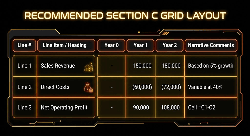
│                        RECOMMENDED SECTION C GRID LAYOUT                               │

├─────────┬──────────────────────┬───────────┬───────────┬───────────┬───────────────────┤

│ Line #  │ Line Item / Heading  │  Year 0   │  Year 1   │  Year 2   │ Narrative Comments│

├─────────┼──────────────────────┼───────────┼───────────┼───────────┼───────────────────┤

│    1    │ Sales Revenue        │     -     │  150,000  │  180,000  │ Based on 5% growth│

│    2    │ Direct Costs         │     -     │  (60,000) │  (72,000) │ Variable at 40%   │

│    3    │ Net Operating Profit │     -     │   90,000  │  108,000  │ Cell =C1-C2       │

└─────────┴──────────────────────┴───────────┴───────────┴───────────┴───────────────────┘

When writing extensive paragraphs, use the built-in Word Processor Response Box if provided alongside the spreadsheet, or type your discussion in dedicated wide text rows below your calculation schedule.

Mistake 5: Neglecting Absolute References ($) for Key Variables

Time management is a major reason candidates fail to complete Section C. A common time-waster is manually re-typing static variable rates (such as inflation, discount rates, or corporate tax rates) into every individual row or column formula.

By mastering Absolute Cell Referencing using the dollar sign ($), you can write a formula once and copy it across 5 years of cash flows in seconds.

Difference Between Relative and Absolute Cell References

• Relative Reference (C4): When you copy the formula to the right (Column D), C4 automatically shifts to D4.

• Absolute Reference (C2): Adding dollar signs locks both the column (C) and row (2). When you copy the formula across Columns D, E, and F, the reference remains locked to C2.

Practical 4-Year Cash Flow Example

Suppose cell C2 contains the annual inflation rate (5.0%), and uninflated sales for Years 1 to 4 are entered in row 5 (D5 to G5).

                   Absolute Referencing ()Mechanics│UninflatedRevenue(Row5)───────┼──────────────►Movesrelatively(D5➔E5➔F5)│InflationRate(C2)───────────┴──────────────►Remainslocked(C$2)

                                                     Formula in Year 1: =D5 * (1 + C2)^1

                                                     Formula in Year 2: =E5 * (1 + C2)^2

Step-by-Step Execution:

1. In Year 1 Inflated Sales cell (D6), type: =D5 * (1 + C2)^1

2. In Year 2 Inflated Sales cell (E6), type: =E5 * (1 + C2)^2

Because C2 is locked with absolute referencing, copying cell D6 across row 6 calculates inflated cash flows for all 4 years without formula errors.

The Ideal Section C Spreadsheet Layout (Master Templates)

To maximize your marks, organize your Section C spreadsheet answers using structured, standardized templates.

1. Financial Reporting (FR): Consolidated Statement Blueprint

========================================================================================

ABC GROUP - CONSOLIDATED STATEMENT OF FINANCIAL POSITION AS AT 31 DECEMBER 20X1

========================================================================================

Line Item                                  Parent (₹)   Sub (₹)    Adjustments (₹)  Group Total (₹)

----------------------------------------------------------------------------------------

Property, Plant & Equipment                450,000     200,000     15,000 (W2)      665,000

Goodwill                                      -           -        42,000 (W3)       42,000

Investments                                 180,000       -       (180,000)(W1)         -

Current Assets                             120,000      85,000      (5,000)(W4)      200,000

----------------------------------------------------------------------------------------

TOTAL ASSETS                                                                     1,107,000

========================================================================================

WORKINGS:

(W1) Group Structure: Parent owns 80% of Sub acquired 1 Jan 20X1.

(W2) Fair Value Adjustment: PPE fair value excess = ₹15,000.

(W3) Goodwill Calculation: Consideration Paid (₹180,000) + NCI (₹38,000) - Net Assets (₹176,000) = ₹42,000.

(W4) Intra-Group Trading: Eliminate inventory unrealized profit (PURP) = ₹5,000.

2. Financial Management (FM): Investment Appraisal Schedule

========================================================================================

PROJECT X - NET PRESENT VALUE (NPV) ANALYSIS (ALL FIGURES IN ₹ '000)

========================================================================================

Cost of Capital: 10% (Cell B2)

Line Item                  Year 0       Year 1       Year 2       Year 3       Year 4

----------------------------------------------------------------------------------------

Initial Outlay            (500,000)        -            -            -            -

Sales Revenue                 -        200,000      250,000      300,000      200,000

Direct Costs                  -       (80,000)    (100,000)    (120,000)     (80,000)

Operating Expenses            -       (30,000)     (35,000)     (40,000)     (30,000)

Tax Payable (30%)             -       (27,000)     (34,500)     (42,000)     (27,000)

Tax Allowed Depreciation      -         15,000       15,000       15,000       15,000

Working Capital           (40,000)     (10,000)     (10,000)       -          60,000

----------------------------------------------------------------------------------------

Net Cash Flow             (540,000)     78,000       95,500      113,000      138,000

----------------------------------------------------------------------------------------

NET PRESENT VALUE (NPV) CALCULATED = ₹(142,350)

Formula used in Cell B15: =NPV(B2, D12:G12) + C12

RECOMMENDATION: Reject Project X as NPV is negative.

3. Performance Management (PM): Variance Analysis & Reconciliation

========================================================================================

OPERATING PROFIT RECONCILIATION STATEMENT FOR THE MONTH ENDED 31 MARCH

========================================================================================

Budgeted Operating Profit                                             ₹120,000

Sales Variances:

  Sales Volume Variance                                   ₹8,000 (F)

                                                          ──────────

Actual Sales at Budgeted Margin                                       ₹128,000

Cost Variances:                               Fav (₹)      Adv (₹)

  Material Price Variance                       -           3,500

  Material Usage Variance                     2,000           -

  Labor Rate Variance                           -           1,800

  Labor Efficiency Variance                   4,500           -

  Fixed Overhead Expenditure Variance           -           2,200

                                              ──────────   ──────────

Sub-totals                                    6,500        7,500       ₹(1,000) (A)

----------------------------------------------------------------------------------------

ACTUAL OPERATING PROFIT                                               ₹127,000

========================================================================================

Essential ACCA CBE Keyboard Shortcuts Cheat Sheet

Efficiency in the exam room relies on muscle memory. Memorize these supported shortcuts to speed up your spreadsheet formatting:

Frequently Asked Questions (FAQs)

1. Will I lose all marks in Section C if my final NPV figure is incorrect?

No, absolutely not. ACCA human markers grade on technique, formula logic, and methodology. If you make a mathematical error in Year 1 sales revenue, but derive your operating profit, tax liabilities, and final NPV using correct dynamic spreadsheet formulas, you will lose only 0.5 or 1 mark for the initial mistake. Full Own Figure Rule (OFR) working marks will be awarded for all subsequent rows.

2. Can I use Microsoft Excel keyboard shortcuts in the official ACCA CBE software?

Most standard editing shortcuts (Ctrl+C, Ctrl+V, Ctrl+Z, Ctrl+B) work identically inside the ACCA CBE environment. However, specialized Excel shortcuts involving function keys (e.g., Alt + = for AutoSum) or complex ribbon navigation shortcuts are unsupported. Always practice inside the official ACCA Practice Platform to master the exact software interface.

3. How do I format negative numbers in the ACCA spreadsheet?

Format negative numbers clearly using either a minus sign (-5000) or standard accounting parentheses (5,000). Whichever convention you choose, apply it consistently throughout your entire response. Surrounding cash outflows in parentheses makes cash flow statements much easier for markers to follow.

4. What happens if I accidentally delete data in my CBE spreadsheet?

Use the keyboard shortcut Ctrl + Z immediately to undo the deletion. If you overwrite a formula or layout, Ctrl + Z will step backward through your edit history.

Master ACCA Exam Technique with Amit Dharaniya

Mastering spreadsheet mechanics and technical accounting frameworks requires structured preparation and professional guidance. If you want to build exam confidence and achieve high scores in your ACCA sittings:

• Explore Expert Guidance & Mentorship: Learn more about Amit Dharaniya's teaching methodology and student performance insights on Amit Dharaniya's Profile.

• Enroll in Professional ACCA Courses: Get immediate access to video lectures, Section C spreadsheet walkthroughs, and practice mocks by visiting Amit Dharaniya's Courses Directory.

Key Takeaways for Section C Distinction

1. Never hardcode calculated numbers—always use live spreadsheet formulas (=SUM, =B4*C4) to protect your method marks under the Own Figure Rule.

3. Format every grid schedule professionally using thousands separators, clear table headers, and bold sub-totals (Ctrl + B).

5. Practice exclusively inside the official ACCA Practice Platform to build speed and accuracy before exam day.Start writing your article...